Convolutional layers of artificial neural networks are analogous to the feature detectors of animal vision in that they both search for pre-defined patterns in a visual field. Convolutional layers form during network training, while the question how animal feature detectors form is a matter of debate. I observed and manipulated developing convolutional layers during training in a simple convolutional network: the MNIST hand-written digit recognition example of Google’s TensorFlow.

Convolutional layers, usually many different in parallel, each use a kernel, which they move over the image like a stencil. For each position the degree of overlap is noted, and the end result is a map of pattern occurrences. Classifier network layers combine these maps to decide what the image represents.

The reason why convolutional layers can work as feature detectors is that discrete convolution, covariance and correlation are mathematically very similar. In one dimension:

Multiply two images pixel-by-pixel, then add up all products to convolve them: $$(f * g)[n] = \sum_{m=-\infty}^\infty f_m g_{(n – m)}$$

Subtract their means E(f) first to instead get their covariance: $$\mathrm{cov} (f,g)=\frac{1}{n}\sum_{m=1}^n (f_m-E(f))(g_m-E(g))$$

Then divide by the variances σ(f) to get their Pearson correlation: $$\mathrm{corr}(f,g)={\mathrm{cov}(f,g) \over \sigma_f \sigma_g} $$

The role of the variable n is to shift the convolution kernel g along the input image. Each time the result is one number, defining one pixel in the output. Then the kernel is shifted by one over the input to calculate the next output pixel. For convolutional layers the kernel proper is finite-length and usually quite short, with zeros assumed everywhere else left and right. The result is a scanning window of interest, because the contribution of the product outside of the kernel proper is zero. It would be easy to add this scanning feature to the covariance and correlation terms. (Note another minor difference: negative m means convolution uses its kernel g backwards.)

The main differences between the three terms are the normalisation for mean and variance. The infinite number of zeros makes both the mean and the variance of a finite-length convolution kernel zero. However if ignoring the artifice of infinite zeros, normalisation becomes meaningful, and potentially useful. If the convolution output is normalised to a fixed output range, then this constitutes a sort-of mean normalisation of kernel and image together. This works best if both are in a similar ranges of values. The result is then somewhat similar to covariance. However, the MNIST example uses neither mean, nor variance normalisation, as would be necessary to obtain the Pearson correlation. (It also does not reverse the kernel, making the convolution operation used more akin to cross-correlation, which is just convolution with a finite length kernel that is not reversed.)

In vivo neurons are likely able to control gain on synapses to normalise mean. Whether they can control variance, and adapt to higher and lower contrast, that to decide is a matter of experiment. If, for example, in a series of pictures with randomly high or low contrast it takes longer to recognise pictures if there was a change of contrast compared to the previous picture, then adaptation takes place. There is certainly some evidence that contrast and overall brightness of an image are handled separately early on in the visual cortex.

In TensorFlow’s MNIST network 32 different 5×5 pixel convolution kernels scan a 28×28 pixels input image of a hand-written digit. The resulting intensity maps go through a RelU operation (which sets everything <0 to 0, eliminating negative values, and introducing a non-linearity). The resulting 32 convolved images are then convolved again with a different set of 32 kernels. The output 1024 images feed (via RelU) into a fully connected neural layer. A linear model uses the output of the fully connected layer to give probabilities which of the digits 0-9 the hand-written input image represents.

The kernels of the first convolution layer start with small random values and are optimised during training with the rest of the network. Given their common purpose, and similar visual experiences during training, I expected that convolutional layers through training form feature detectors similar to animal vision. I assumed they would become sensitive to lines at different angles, edges, and perhaps curves. The random seed values were around 0 with a standard deviation of 0.1, while the input image brightness was encoded with values between 0 and 1.

Instead of forming recognisable feature detectors, the initially random kernels hardly changed during all training, despite digit recognition accuracy increasing to the expected 99.2%. The magnitude of change per pixel remained very small throughout optimisation of both sets of kernels, about 0.0005, or 1/200 of the standard deviation of the initial random values. Even this must have involved much back-and-forth as the overall change through 20 000 cycles of training remained minimal. The random kernel patterns at the beginning of training were nearly indistinguishable from those at the end of training. Using the kernels to convolve the same input yielded very nearly identical results. Nonetheless, despite a different random kernel in each training run, recognition accuracy reliably reached the same high result. This was unexpected.

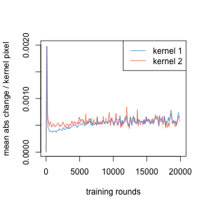
The absolute change of kernel pixel values per 100 cycles of optimisation was very small compared to the image (0-1) and the kernel initial range (mean 0, sd 0.1) of values. This was true for both the kernel sets of the first and second convolutional layers.

This suggested that the first kernels do not need to have any particular shape at all. Indeed, any set of random kernels in the first convolutional layer, without optimising, was sufficient to reach 99.2% accuracy. The training improvement was indistinguishable whether the first kernels were optimised, or held constant from the beginning. Only when both convolution layers remained unoptimised did learning slow down, and final accuracy decrease to 98.6%.

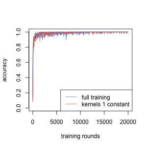
Training accuracies develop the same both with optimised and constant convolution kernels (3 optimised, 2 unoptimised runs)

(To be continued … )